Digital Image Processing | Histogram Calculation, Equalization and Normalization

This article continues the basics of the digital image processing series. In this article, I will talk about histogram calculation and equalization.

So, what is the histogram? The histogram represents the intensity level of each color in a digital image.

Why do we need histogram calculation? The histogram calculation allows us to think about thresholds that can used to filter images or extract information from images.

Why do we need histogram equalization? Histogram equalization helps us get a more pleasurable digital image.

Please note that the result of histogram calculation is always a curve; the result of histogram equalization is the image.

Before executing the provided code, ensure you have installed Python packages for OpenCV, NumPy, and PyPlot.

Histogram calculation and equalization

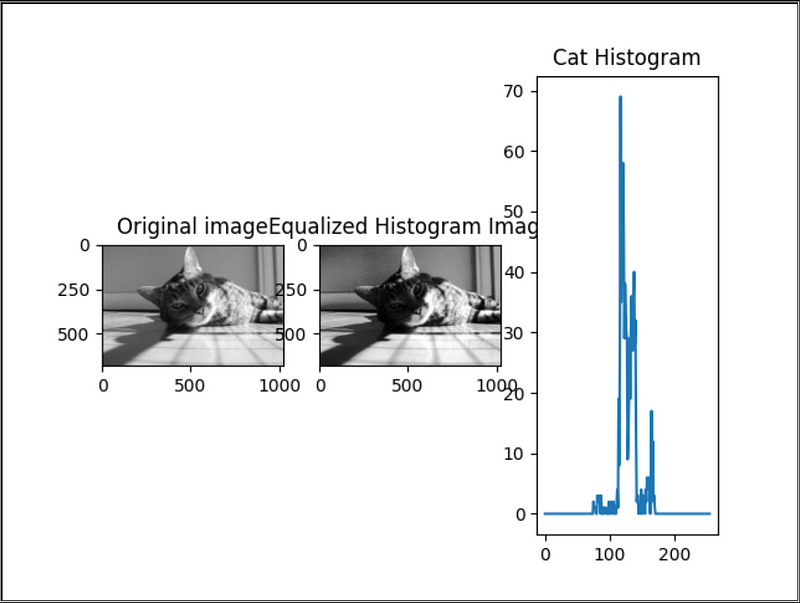
I will be using the following image.

import cv2 
from matplotlib import pyplot as pt 
 
cat = cv2.imread("img/cat.jpg", 0) 
cat_equalized = cv2.equalizeHist(cat) 
cat_hist = cv2.calcHist(cat, [0], None, [256], [0, 256]) 
 
pt.figure() 
pt.tight_layout() 
pt.subplot(1, 3, 1) 
pt.title("Original image") 
pt.imshow(cat, cmap='gray') 
 
pt.subplot(1, 3, 2) 
pt.title("Equalized Histogram Image") 
pt.imshow(cat_equalized, cmap='gray') 
 
pt.subplot(1, 3, 3) 
pt.plot(cat_hist) 
pt.title('Cat Histogram') 
pt.show() 
 
cv2.waitKey() 
cv2.destroyAllWindows()

As you can see, it is pretty simple — use methods provided by the OpenCV library.

Be aware that the method imshow from Pyplot cannot work as expected if you are not specifying a color map. In the provided example above, the color map is gray.

Histogram Normalization

Accoding Scientific Computing and Imaging Institute

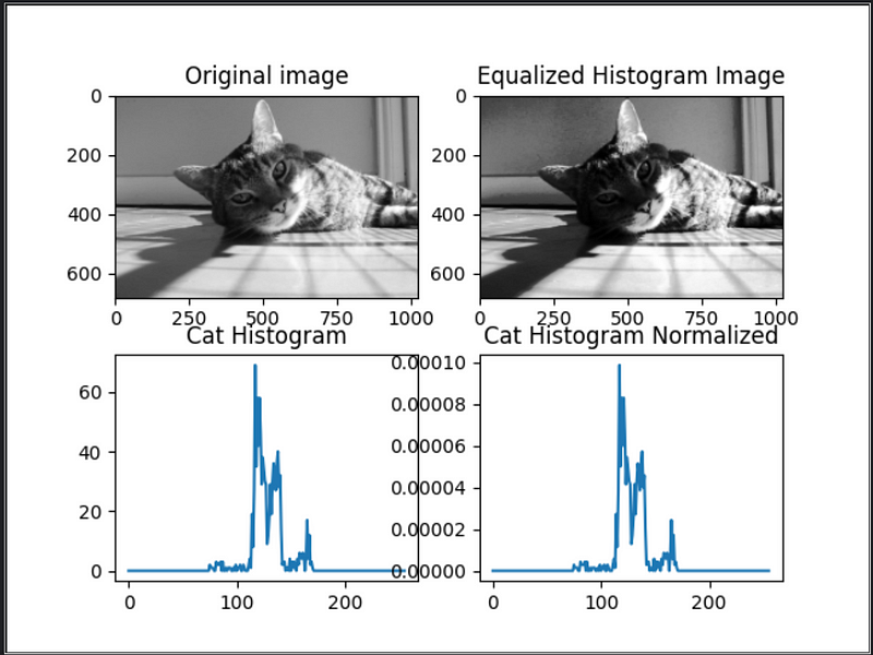
Normalize an histogram is a technique consisting into transforming the discrete distribution of intensities into a discrete distribution of probabilities. To do so, we need to divide each value of the histogram by the number of pixel.

The process of histogram normalization is quite simple; we have to divide the equalized histogram by the total number of pixels.

import cv2 
from matplotlib import pyplot as pt 
 
cat = cv2.imread("img/cat.jpg", 0) 
[n_row, n_col] = cat.shape 
total_no_pixels = n_row * n_col 
cat_equalized = cv2.equalizeHist(cat) 
cat_hist = cv2.calcHist(cat, [0], None, [256], [0, 256]) 
cat_hist_normalized = cat_hist / total_no_pixels 
 
pt.figure() 
pt.tight_layout() 
pt.subplot(2, 2, 1) 
pt.title("Original image") 
pt.imshow(cat, cmap='gray') 
 
pt.subplot(2, 2, 2) 
pt.title("Equalized Histogram Image") 
pt.imshow(cat_equalized, cmap='gray') 
 
pt.subplot(2, 2, 3) 
pt.plot(cat_hist) 
pt.title('Cat Histogram') 
 
pt.subplot(2, 2, 4) 
pt.plot(cat_hist_normalized) 
pt.title('Cat Histogram Normalized') 
pt.show() 
 
cv2.waitKey() 
cv2.destroyAllWindows()

As you can see at the bottom right corner, the range values have been scaled to less range.

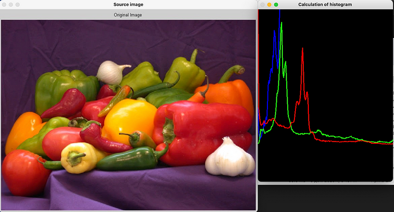
Please remember that the grayscale and binary images contain only one plane of pixels, and RGB consists of 3 planes. One plane for each color

Take note that the OpenCV library reads images into different orders of planes. It is not RGB, it is BGR

import cv2 as cv 
import numpy as np 
 
src = cv.imread("orginal.jpg") 
 
bgr_planes = cv.split(src) 
hist_size = 256 
hist_range = (0, 256)  # the upper boundary is exclusive 
 
r_hist = cv.calcHist(bgr_planes, [0], None, [hist_size], hist_range, accumulate=False) 
g_hist = cv.calcHist(bgr_planes, [1], None, [hist_size], hist_range, accumulate=False) 
b_hist = cv.calcHist(bgr_planes, [2], None, [hist_size], hist_range, accumulate=False) 
 
hist_width = 512 
hist_height = 400 
bin_weight = int(round(hist_width / hist_size)) 
 
hist_image = np.zeros((hist_width, hist_height, 3), dtype=np.uint8) 
 
cv.normalize(r_hist, r_hist, alpha=0, beta=hist_height, norm_type=cv.NORM_MINMAX) 
cv.normalize(g_hist, g_hist, alpha=0, beta=hist_height, norm_type=cv.NORM_MINMAX) 
cv.normalize(g_hist, g_hist, alpha=0, beta=hist_height, norm_type=cv.NORM_MINMAX) 
 
for i in range(1, hist_size): 
    cv.line(hist_image, (bin_weight * (i - 1), hist_height - int(b_hist[i - 1])), 
            (bin_weight * i, hist_height - int(b_hist[i])), 
            (255, 0, 0), thickness=2) 
    cv.line(hist_image, (bin_weight * (i - 1), hist_height - int(g_hist[i - 1])), 
            (bin_weight * i, hist_height - int(g_hist[i])), 
            (0, 255, 0), thickness=2) 
    cv.line(hist_image, (bin_weight * (i - 1), hist_height - int(r_hist[i - 1])), 
            (bin_weight * i, hist_height - int(r_hist[i])), 
            (0, 0, 255), thickness=2) 
 
cv.imshow('Source image', src) 
cv.imshow('Calculation of histogram', hist_image) 
cv.waitKey()

References

1. OpenCV tutorial
2. Rafael C. Gonzalez • Richard E. Woods, Digital Image Processing
3. Scientific Computing and Imaging Institute
4. Digital Image Processing Basics